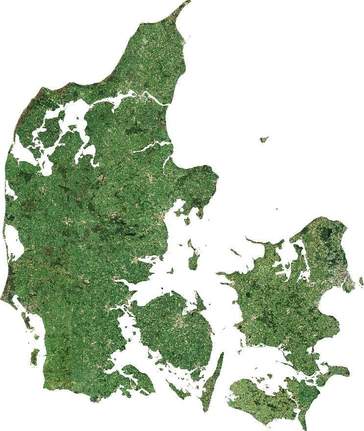
Creating mosaics from Sentinel 2 satellite imagery

Prerequisites

First, some satellite imagery is needed, and there are several ways to get this. Here, I have used images from the Sentinel 2A and 2B missions which provide high resolution (10 m) RGB imagery. Furthermore, the data are available with different levels of pre-processing (Level 2A is used here). The data can be downloaded from the Copernicus Open Access Hub through an API or interactive GUI. Here, 105 (83 GB) low cloud-cover images covering the period from start May to end September 2020.

Also, a polygon of Denmark is downloaded and processed with the raster and sf packages, and will be used to mask out the ocean and coastal waters:

#Download polygon of Denmark
library(raster)
library(sf)
dk_border_raw <- getData("GADM", country = "DNK", level = 0, 
                         path = paste0(getwd(), "/data/sentinel_processed"))

dk_border <- dk_border_raw |>
  st_as_sf() |> 	
  st_crop(xmin = 8, ymin = 54.56, xmax = 14, ymax = 57.76) |> 	
  st_transform(25832)	

st_write(dk_border, paste0(getwd(), "/data/sentinel_processed/dk_border.sqlite"))

dk_bbox <- st_bbox(dk_border)

Create initial mosaic

The gdalcubes package uses image collections which can be created by pointing it to a folder containing the downloaded ‘.zip’ files. From this image collection, a view is defined, setting the temporal and spatial resolution. Overlapping pixels are aggregated by the median and the mask band included in the raw data is also used to mask out clouds. In essence, 14 day image mosaics are created which are then again aggregated by the 1st quantile which results in a good looking mosaic. These are the main steps defined in the processing pipeline, and the mosaic can finally be written to a ‘.tif’ file:

#Load gdalcubes library
library(gdalcubes)

#Set number of cores to be used
gdalcubes_options(threads = 8)

#Get list of files sentinel 2 files (.zip archives)
#May look something like: 
#S2A_MSIL2A_20200507T104031_N0214_R008_T32UPF_20200507T112418.zip
sentinel_folder <- paste0(getwd(), "/data/sentinel/")
sentinel_files <- list.files(sentinel_folder, pattern = "*.zip", full.names = TRUE)

#Create image collection from files
create_image_collection(sentinel_files, 
                        format="Sentinel2_L2A", unroll_archives=TRUE, 
                        out_file=paste0(getwd(), "/data/sentinel_processed/sentinel2.db")) 

img_collection <- image_collection(paste0(getwd(), "/data/sentinel_processed/sentinel2.db"))

#Define view of datacube i.e. spatial and temporal extent
img_view <- cube_view(srs="EPSG:25832", 
                      extent=list(left=dk_bbox[["xmin"]], right=dk_bbox[["xmax"]], 
                                  bottom=dk_bbox[["ymin"]], top=dk_bbox[["ymax"]],
                                  t0 = "2020-05-01", t1 = "2020-09-30"),
                      dx=10,
                      aggregation = "median",
                      resampling = "bilinear",
                      dt = "P14D")

#Define mask values (mask band included with sentinel 2 L2A data)
img_mask <- image_mask("SCL", values = c(3, 8, 9))

#Define function for calculting the 1st quantiles
q25_band <- function(x){
  c(quantile(x["B04", ], 0.25, na.rm=TRUE),
    quantile(x["B03", ], 0.25, na.rm=TRUE),
    quantile(x["B02", ], 0.25, na.rm=TRUE))
}

img_cube <- raster_cube(image_collection=img_collection, 
            view=img_view,
            mask=img_mask,
            chunking=c(1, 1024, 1024)) |>
  select_bands(c("B02", "B03", "B04")) |>
  reduce_time(names=c("q25_red", "q25_green","q25_blue"), FUN = q25_band)

write_tif(img_cube,
          dir = paste0(getwd(), "/data/sentinel_processed/"), 
          prefix = "mosaic_", 
          creation_options = list("COMPRESS" = "LZW", "BIGTIFF" = "YES"))

Further processing

The initial mosaic contains both land and water but using the polygon that was downloaded, the ocean and coastal waters can be removed. Also, the datatype in the initial mosaic is floating point, and to reduce file size, it is converted to byte type and in turn a ‘.png’ file. All this image processing is done using the GDAL command-line tools through the gdalUtils package:

#Further processing of mosaic using GDAL 
library(gdalUtils)

#Mask mosaic by country shape
gdalwarp(paste0(getwd(), "/data/sentinel_processed/mosaic_2020-05-01.tif"),
         paste0(getwd(), "/data/sentinel_processed/mosaic_2020_masked.tif"), 
         cutline = paste0(getwd(), "/data/sentinel_processed/dk_border.sqlite"),
         crop_to_cutline = TRUE,
         co = c("COMPRESS=LZW", "BIGTIFF=YES"),
         multi=TRUE)

#Convert to byte by histogram stretching
#Use a reasonable default value for all bands (e.g. 1250 as here),
#experiment with other values, or compute band stats (e.g. gdalinfo) and 
#use quantiles on a per band basis.
gdal_translate(src_dataset = paste0(getwd(), "/data/sentinel_processed/mosaic_2020_masked.tif"),
               dst_dataset = paste0(getwd(), "/data/sentinel_processed/mosaic_2020_masked_byte.tif"),
               ot = "Byte",
               scale = c(1, 1250, 0, 255),
               co = c("COMPRESS=LZW", "PHOTOMETRIC=RGB"))

#Create .png file
gdal_translate(src_dataset = paste0(getwd(), "/data/sentinel_processed/mosaic_2020_masked_byte.tif"),
               dst_dataset = paste0(getwd(), "/data/sentinel_processed/mosaic_2020.png"),
               of = "PNG",
               outsize = c("2.5%", "2.5%"))

This processsing results in the final image mosaic (drastically downscaled), and is an ‘average’ image of the 2020 summer:

Concluding remarks

Making high resolution image mosaics is simple in R using the presented packages. The gdalcubes package also makes it simple to create ‘.gif’ files which is a neat way to present the temporal dimension of the data. There are many potential applications for this type of data which exists and is freely available in large quantities. While the spatial dimension presents interesting use cases, the temporal dimension might present particularly interesting information. Satellite imagery are used for an increasing number of purposes making it a very interesting field to follow!