Bathymetric maps and interpolation with R

Get some data!

As input data, two things are needed: lake depths measured at geographic coordinates and a lake boundary polygon. I use Danish monitoring data which are publicly available from the surface water database ODA. The depth measurements are performed as a part of the plant monitoring program. For some lakes, this result in a lack of coverage over deep parts of a lake where plants are unlikely to grow. The lake boundary polygons are available from ‘Kortforsyningen’. All the required data are freely available and bathymetric maps may be of interest to wide range of people from researchers to anglers and naturalists. As an example, I have downloaded data from the southern basin of Lake Filsø.

Getting the data in shape

Raw depth data (ODA->Hent data->Sø->Vegetation->Transekt - punkt) and lake polygons (DK_StandingWater layer) are downloaded and imported into R. We do some initial processing and end up with a spatial point vector containing X-Y coordinates and measured depth with 0 depth along the lake boundary:

library(raster);library(sf);library(tidyverse);library(fields);library(readxl);library(interp);library(leaflet)

#Load excel file and rename columns
#Convert column with depths to numeric and covert to unit meter
raw_df <- read_excel("filsø.xlsx") %>% 
  mutate(z = parse_number(`Vanddybden i m`)/100) %>% 
  select(x = `Punkt X-UTM`, y = `Punkt Y-UTM`, z)

#Use sf to convert raw_df to spatial point vector
#Coordinate reference system is UTM zone 32, EUREF89, with EPSG code 25832
lake_depth_xyz <- raw_df %>% 
  st_as_sf(coords = c("x", "y"), crs = 25832)

#Get centroid for joining with polygon
lake_centroid <- st_centroid(st_union(lake_depth_xyz))

#Load lake polygons (large file with 179242 features
dk_lake_polygons <- st_read("DK_StandingWater.gml") 

#Get polygon id (gml_id) for Filsø (Søndersø) by spatial intersection
lake_polygon_id <- st_intersection(dk_lake_polygons, lake_centroid)

#Extract polygon
lake_polygon <- dk_lake_polygons %>% 
  filter(gml_id == lake_polygon_id$gml_id)

#The lake_polygon is converted to a line vector in order to sample (25 points/km) points where depth equals zero
lake_border_xyz <- lake_polygon %>% 
  st_cast("MULTILINESTRING") %>% 
  st_cast("LINESTRING") %>% 
  st_line_sample(density = 0.025) %>% 
  st_cast("POINT") %>% 
  st_as_sf() %>% 
  mutate(z = 0) %>% 
  rename(geometry = x)

#Finally the all depths measurements are joined
#The second argument ensures that only depth measurements within the lake polygon is used
lake_xyz <- rbind(lake_border_xyz, 
      st_intersection(lake_depth_xyz, lake_polygon$geometry))

That is the data preparation necessary in order to perform the interpolation. Lets just visualize the data before exploring options for interpolation.

pal <- colorNumeric(palette = "magma", lake_xyz$z)

lake_xyz %>% 
  st_transform(4326) %>% 
  as("Spatial") %>% 
  leaflet() %>% 
  addTiles() %>% 
  addCircles(color = ~pal(z)) %>% 
  addLegend(pal = pal, values = ~z, title = "Lake depth (m)", opacity = 1)

For relatively sparse data as this with around 300 measurements across a large lake, simple methods such as piece-wise linear interpolation often do well. This method assumes nothing and interpolates only within the given area and data range. We also try out a more flexible method, a thin-plate spline smoother, which produces results which are visually much nicer. However, it may yield unexpected results but it depends on the data, if the depth has been measured regularly across the lake it should be alright. Other interpolation methods such as inverse-distance-weighted does generally not do so well on this kind of better but may be more appropriate for filling small holes in more densely sampled surfaces (link to another comparison of methods in R).

#We try two interpolation methods: piece-wise interpolation in the interp package and thin-plate spline in fields package
#First create an empty raster to interpolate over, adjust resolution depending on lake and computer power
tmp_raster <- raster(lake_xyz, res = c(5, 5), crs = st_crs(lake_xyz)$proj4string)

#First the simpler linear interpolation 
#Input data and dimensions of the output grid are provided
linear <- interp(as(lake_xyz, "Spatial"),
                 z = "z",
                 ny=ncol(tmp_raster),
                 nx=nrow(tmp_raster),
                 duplicate = "mean")

#Convert to raster object and resample to resolution in tmp_raster
linear_warp <- resample(raster(linear), tmp_raster)

#Mask by lake polygon
linear_mask <- mask(linear_warp, as(lake_polygon, "Spatial"))

#Next, the more flexible smooth thin-plate spline smoothing method
#Fit function
tps_fun <- Tps(st_coordinates(lake_xyz), lake_xyz$z)

#Use to interpolate on the empty
tps <- interpolate(tmp_raster, tps_fun)

#Set a few negative values to zero and change layer name
tps[tps < 0] <- 0 
names(tps) <- "z"

tps_mask <- mask(tps, as(lake_polygon, "Spatial"))

#Contour lines kan also be created for each 0.5 meters for example
linear_contour <- rasterToContour(linear_mask, 
                                  levels = seq(0, round(max(linear_mask[], na.rm = TRUE)), 0.5))

tps_contour <- rasterToContour(tps_mask,
                               levels = seq(0, round(max(tps_mask[], na.rm = TRUE)), 0.5))

#Lets plot the difference of the two methods
as.data.frame(linear_mask-tps_mask, xy = TRUE) %>% 
  ggplot()+
  geom_raster(aes(x, y, fill = layer))+
  geom_sf(data = lake_polygon, fill = NA, col = "black", size = 1)+
  scale_fill_gradient2(low = "blue", high = "coral", mid = "grey", na.value = "white", name = "Depth (m)")+
  theme_void()+
  guides(fill=guide_colorbar(title.position = "top"))+
  theme(legend.position = "bottom")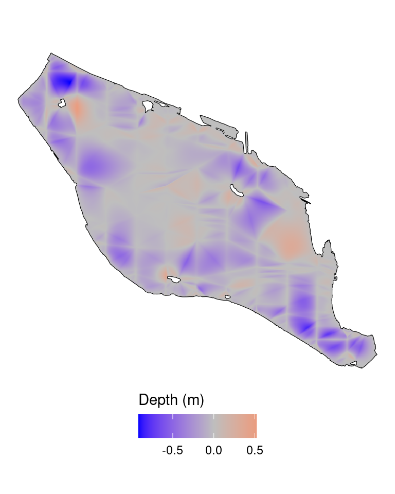

Notice the differences in the depth interpolated by the two methods. Red regions are where the linear interpolation is higher than the tps and blue regions vice versa. The tps smoother are extrapolating beyond the measured depth data points.

That was the number-crunching part, lets visualize the resulting maps.

#Convert rasters to data frame with an additional column identifying method and spatial objects to sf for plotting with ggplot
bathy_df <- bind_rows(as.data.frame(linear_mask, xy = TRUE) %>% add_column(method = "Linear interpolation"),
                      as.data.frame(tps_mask, xy = TRUE) %>% add_column(method = "Tps interpolation"))

contour_sf <- rbind(st_as_sf(linear_contour) %>% add_column(method = "Linear interpolation"),
                    st_as_sf(tps_contour) %>% add_column(method = "Tps interpolation"))

#Plot interpolated rasters with contour lines and lake boundary
bathy_df %>% 
  ggplot()+
  geom_raster(aes(x, y, fill = z))+
  scale_fill_viridis_c(na.value = "white", name = "Depth (m)", option = "A",
                       trans = "reverse", direction =-1, begin = 0.2)+
  geom_sf(data = contour_sf, linetype = 2)+
  geom_sf(data = lake_polygon, fill = NA, col = "black", size = 1)+
  facet_grid(.~method)+
  theme_void()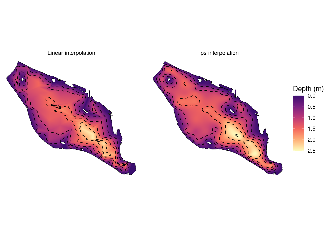

Whats next?

As showed in this example, some choices regarding interpolation method must be made which most often depend on the data. If in doubt, the simplest approach is often the most sensible. This example shows that R has good tools available for fast experimentation but for rich data-sets spanning a large geographical region other options are also available. GDAL provide command-line tools to do this which is something I will show in another post. By saving the resulting maps as .kml/.kmz files they can also be viewed in Google Earth on a phone along with your current position. This is a nice feature if the maps are needed for field work or other recreative activities.